Fundamentals of state space design.

1.  Understanding time

1.1 Introduction to the module.

The purpose of this module is to warm you up to the more advanced modules that will follow.  It is not to scare you with a heap of new concepts and tricks.  Although, of course, you might already be familiar with them.

You will find quite a few JavaScript demonstrations to play with – and playing with them is an important part of this module.  You can regard their details as mysteries to be revealed by those later modules, or as something to pry into out of curiosity.  The assessment will be based much more on gathering your impressions of them than on any ability to perform party tricks.

Enjoy!

1.2  It’s about time.

Many books on control theory are filled with block diagrams and polynomials in ‘s’.

The world is not like that.  

We must open those block diagram boxes and look inside.

Everything that changes has a ‘state’ that tells you something about it, right now.

If you open your hand to drop a ball, one of its ‘state variables’ is its height above the floor, let us call that ‘y’.  Another is the velocity at which it is falling, which we might call ‘vy’.

But as time passes, those variables will change, and we will be curious about how to predict the new values.  To help us do that, we need to know their rate-of-change, and these will be differential equations in time.

For our ball, the rate of change of height y is the vertical velocity vy, so we have the rather obvious equation

$\frac{d}{\mathit{dt}}\left(y\right)=\mathit{vy}$

But vy is changing too, and ignoring any air resistance, it has its own equation

$\frac{d}{\mathit{dt}}\left(\mathit{vy}\right)=g$

Here g is the acceleration due to gravity, with a value -9.8 metres/sec/sec.

Though the equations look very simple, we can do a lot with them, including creation of a dynamic picture.  The details will have to wait until the module on simulation,

• but click on this link.

Maybe you have tossed the ball with a horizontal velocity, so that the rate of change of horizontal position x is vx

$\frac{d}{\mathit{dt}}\left(x\right)=\mathit{vx}$

and we can consider an unnecessary equation

$\frac{d}{\mathit{dt}}\left(\mathit{vx}\right)=0$

So the behaviour is now like this

1.3  Integrators and notation

The ‘engine room’ of any simulation is a set of integrators.  These can be electronic devices involving operational amplifiers and capacitors, or mere lines of software to track the travels of the state variables as ruled by the state equations.  

Rather than write the cumbersome d/dt in these equations, we denote a derivative by putting a dot over the variable, or a double dot if it is a second derivative.  So our equations above become

$\dot{y}=\mathit{vy}$

$\dot{\mathit{vy}}=g$

$\dot{x}=\mathit{vx}$

$\dot{\mathit{vx}}=0$

We could have written

$\ddot{y}=g$

but this would not give us an equation with which to track the vertical velocity.

So state equations are always first order, giving us the means to work out what the values of the state variables will be a moment later.

In school, the meaning of differentiation was drilled into you, by considering $\dot{x}$  as the limit of

$\frac{x\left(t+\mathit{\delta t}\right)-x\left(t\right)}{\mathit{\delta t}}$

as $\delta t$  tends to zero.  

Now we can  turn that around, as the limit of

$x\left(t+\mathit{\delta t}\right)=x\left(t\right)+\dot{x}\ast \mathit{\delta t}$

when $\delta t$  tends to zero.  But for engineering purposes, we can just make $\delta t$  ‘small enough’.

Of course this will involve an approximation, since vx can be changing over the interval, so dt must be made very small in a line of code

x=x+vx*dt

This will update the value of x right now, to be the value that it will take a moment dt later.  To check whether dt is really small enough, we can halve it and see if that makes any visible difference to the solution.

1.4  A position control example

Let us consider the following design brief.

A mass of 1 kg must be moved to a new position, one metre away, settling to within 1 mm accuracy within a time of one second.  The position control must be stiff, so that a disturbing force of one Newton will not deflect the mass by more than 1 mm from the target position.

Where should the designer start?

Let us ignore details such as the motor inertia, and just regard the motor as applying an acceleration to the mass, maybe by driving a belt.

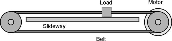
The first task is to choose a suitable motor.  What acceleration is needed for the mass to make its journey in one second?

Assuming that the limits ±amax of acceleration and deceleration are equal in magnitude, the mass must make half its journey in under half a second while accelerating, taking another half second to come to rest.

So

  $\frac{1}{2}\mathit{amax}{t}^2=\frac{1}{2}$ ,

where t = $\frac{1}{2}$  second.

amax = 4 m/s2

To be safe, let us choose a motor that gives 10 m/s2, that is 1 kg force.

The first thing on a control engineer’s mind is feedback. The motor must be driven with an input drive, with some value based on the state variables and their desired target.  The limit on this feedback value can be set at 1, so that with the chosen motor,

$\ddot{x}=10\ast \mathit{drive}$ ,

where |drive|<1.

We have state equations to tell us how x will respond, but we have to make decisions about the input, drive.

1.5  Feedback

If we want to move the mass to a target position target, we might start by applying the error to the drive.  In code form, writing u for 10*drive, this would be

u=k*(target-x)

Does this work?  

Let us make the target zero, and put the initial position one metre away, at x = 1.  Let us try k = 6, so our state equations become:

$\dot{x}=\mathit{vx}$

$\dot{\mathit{vx}}=u$ ,

where u = 6*(target - x)

As a second-order equation, this is

$\ddot{x}=-6\ast x$

To see it in action, click here.

We clearly need some velocity feedback

Let us try

u=6*(target-x)–5*vx

This could be written as a second-order equation

$\ddot{x}+5\ast \dot{x}+6\ast x=6\ast \mathit{target}$

Click here to see the result.  It might look acceptable, but there is much more to consider.